Harry Potter NLP 1

Basic text analysis for:
Harry Potter and the Philosopher’s Stone (1997)
Harry Potter and the Chamber of Secrets (1998)
Harry Potter and the Prisoner of Azkaban (1999)
Harry Potter and the Goblet of Fire (2000)
Harry Potter and the Order of the Phoenix (2003)
Harry Potter and the Half-Blood Prince (2005)
Harry Potter and the Deathly Hallows (2007)

Bottom Line Up Front

Below is a high level, natural language processing (NLP) analysis of the Harry Potter Series. It seeks to find answers to the questions:

• Which book has a bigger vocab?
• Who is Harry’s closest friend?
• Who are the most prominent secondary characters?
• What are the 4 major themes/settings in the Series?

It finds that:

Vocab
Each subsequent book increased its count of unique words. However, Goblet of Fire (Book 4) is a notable exception with the second most unique words. Meanwhile, Order of the Phoenix (Book 5) contains the most repetitive vocabulary.

Best Friend
Ron is Harry’s closest friend, although Hermoine’s friendship grows throughout the Series.

Secondary Characters
Professor Dumbledore is the most prominent secondary character throughout the books, while the new teachers at Hogwarts are the most prominent within 5 of the 7 books. Four of these times, the new teacher is the Defense Against the Dark Arts teacher.

Major Themes/Settings
The Muggle world, the magical community outside Hogwarts, Voldemort’s story arch, and the Hogwarts classroom/Quidditch field are the 4 broadest themes/settings.

Setup

rm(list = ls())
gc()


# install.packages('pacman') install.packages('remotes') library(remotes)
# install.packages('devtools') library(devtools) library(magrittr)
# devtools::install_github('wch/webshot') webshot::install_phantomjs()
# library(BiocManager)
# BiocManager::install('https://bioconductor.org/biocLite.R')
# source('https://bioconductor.org/biocLite.R') biocLite('EBImage')
library(pacman)
pacman::p_load(devtools, knitr, magrittr, dplyr, ggplot2, text2vec, tm, tidytext, 
    stringr, stringi, SnowballC, stopwords, wordcloud, prettydoc, cowplot, kable, 
    utf8, corpus, glue, topicmodels, stm, wordcloud2, htmlwidgets, viridis)

knitr::opts_chunk$set(echo = TRUE, message = FALSE, comment = NA, warning = FALSE, 
    tidy = TRUE, results = "hold", cache = FALSE, dpi = 120)

# Parameters N-gram
ngrams <- "single words"
ngram <- c(1, 1)

## Number of Topics
K <- 4

# Custom functions Remove quotation marks
pasteNQ <- function(...) {
    output <- paste(...)
    noquote(output)
}
pasteNQ0 <- function(...) {
    output <- paste0(...)
    noquote(output)
}

## Chart Template
Grph_theme <- function() {
    palette <- brewer.pal("Greys", n = 9)
    color.background = palette[2]
    color.grid.major = palette[3]
    color.axis.text = palette[6]
    color.axis.title = palette[7]
    color.title = palette[9]
    theme_bw(base_size = 9) + theme(panel.background = element_rect(fill = color.background, 
        color = color.background)) + theme(plot.background = element_rect(fill = color.background, 
        color = color.background)) + theme(panel.border = element_rect(color = color.background)) + 
        theme(panel.grid.major = element_line(color = color.grid.major, size = 0.25)) + 
        theme(panel.grid.minor = element_blank()) + theme(axis.ticks = element_blank()) + 
        theme(legend.position = "none") + theme(legend.title = element_text(size = 16, 
        color = "black")) + theme(legend.background = element_rect(fill = color.background)) + 
        theme(legend.text = element_text(size = 14, color = "black")) + theme(strip.text.x = element_text(size = 14, 
        color = "black", vjust = 1)) + theme(plot.title = element_text(color = color.title, 
        size = 20, vjust = 1.25)) + theme(axis.text.x = element_text(size = 14, color = "black")) + 
        theme(axis.text.y = element_text(size = 14, color = "black")) + theme(axis.title.x = element_text(size = 16, 
        color = "black", vjust = 0)) + theme(axis.title.y = element_text(size = 16, 
        color = "black", vjust = 1.25)) + theme(plot.margin = unit(c(0.35, 0.2, 0.3, 
        0.35), "cm"))
}

## Chart Template Facet Wrap
Grph_theme_facet <- function() {
    palette <- brewer.pal("Greys", n = 9)
    color.background = palette[2]
    color.grid.major = palette[3]
    color.axis.text = palette[6]
    color.axis.title = palette[7]
    color.title = palette[9]
    theme_bw(base_size = 9) + theme(panel.background = element_rect(fill = color.background, 
        color = color.background)) + theme(plot.background = element_rect(fill = color.background, 
        color = color.background)) + theme(panel.border = element_rect(color = color.background)) + 
        theme(panel.grid.major = element_line(color = color.grid.major, size = 0.25)) + 
        theme(panel.grid.minor = element_blank()) + theme(axis.ticks = element_blank()) + 
        theme(legend.position = "none") + theme(legend.title = element_text(size = 11, 
        color = "black")) + theme(legend.background = element_rect(fill = color.background)) + 
        theme(legend.text = element_text(size = 9, color = "black")) + theme(strip.text.x = element_text(size = 9, 
        color = "black", vjust = 1)) + theme(plot.title = element_text(color = color.title, 
        size = 20, vjust = 1.25)) + theme(axis.text.x = element_text(size = 9, color = "black")) + 
        theme(axis.text.y = element_text(size = 9, color = "black")) + theme(axis.title.x = element_text(size = 10, 
        color = "black", vjust = 0)) + theme(axis.title.y = element_text(size = 10, 
        color = "black", vjust = 1.25)) + theme(plot.margin = unit(c(0.35, 0.2, 0.3, 
        0.35), "cm"))
}

## Clean Corpus
cleancorpus <- function(rawtext, remove = NULL, retain = NULL) {
    # Set to lowercase
    rawtext <- tolower(rawtext)
    print(pasteNQ("Set to lowercase"))
    
    # Remove contractions
    fix_contractions <- function(rawtext) {
        rawtext <- gsub("will not", "won't", rawtext)
        rawtext <- gsub("can't", "cannot", rawtext)
        rawtext <- gsub("can not", "cannot", rawtext)
        rawtext <- gsub("shall not", "shant", rawtext)
        rawtext <- gsub("n't", " not", rawtext)
        rawtext <- gsub("'ll", " will", rawtext)
        rawtext <- gsub("'re", " are", rawtext)
        rawtext <- gsub("'ve", " have", rawtext)
        rawtext <- gsub("'m", " am", rawtext)
        rawtext <- gsub("'d", " would", rawtext)
        rawtext <- gsub("'ld", " would", rawtext)
        rawtext <- gsub("'ld", " would", rawtext)
        rawtext <- gsub("'s", "", rawtext)
        return(rawtext)
    }
    rawtext <- fix_contractions(rawtext)
    print(pasteNQ("Fixed contractions"))
    
    # Remove puncutation, numbers, and other none characters
    rawtext <- removePunctuation(rawtext)
    rawtext <- removeNumbers(rawtext)
    rawtext <- gsub("[^[:alnum:]///' ]", "", rawtext)
    rawtext <- gsub("[']", "", rawtext)
    print(pasteNQ("Removed punctuation, numbers, and other none characters"))
    
    # Strip whitespace
    rawtext <- stripWhitespace(rawtext)
    print(pasteNQ("Stripped whitespace"))
    
    # Stemming words
    rawtext <- stemDocument(rawtext)
    print(pasteNQ("Stemmed words"))
    
    return(rawtext)
}

# Remove stop words
removestopwords <- function(rawtext, remove = NULL, retain = NULL) {
    
    # Remove stop words
    stopwords_custom <- stopwords::stopwords("en", source = "snowball")
    stopwords_custom <- c(stopwords_custom, remove)
    stopwords_retain <- retain
    stopwords_custom <- stopwords_custom[!stopwords_custom %in% stopwords_retain]
    rawtext <- removeWords(rawtext, stopwords_custom)
    print(pasteNQ("Removed", length(stopwords_custom), "stop words"))
    
    return(rawtext)
}

# Remove JavaScript from WordClouds
library("EBImage")
embed_htmlwidget <- function(widget, rasterise = T) {
    outputFormat = knitr::opts_knit$get("rmarkdown.pandoc.to")
    if (rasterise || outputFormat == "latex") {
        html.file = tempfile("tp", fileext = ".html")
        png.file = tempfile("tp", fileext = ".png")
        
        htmlwidgets::saveWidget(widget, html.file, selfcontained = FALSE)
        webshot::webshot(html.file, file = png.file, vwidth = 700, vheight = 500, 
            delay = 10)
        img = EBImage::readImage(png.file)
        EBImage::display(img)
    } else {
        widget
    }
}

Load Data

We start by loading in each of the 7 Harry Potter books in which each row represents a chapter.

# devtools::install_github('bradleyboehmke/harrypotter')
library(harrypotter)

titles <- c("Philosopher's Stone", "Chamber of Secrets", "Prisoner of Azkaban", "Goblet of Fire", 
    "Order of the Phoenix", "Half-Blood Prince", "Deathly Hallows")

# lapply(titles, data)
books <- list(philosophers_stone, chamber_of_secrets, prisoner_of_azkaban, goblet_of_fire, 
    order_of_the_phoenix, half_blood_prince, deathly_hallows)

# Save entire corpus
corpus <- c(philosophers_stone, chamber_of_secrets, prisoner_of_azkaban, goblet_of_fire, 
    order_of_the_phoenix, half_blood_prince, deathly_hallows)

# Save df with chapter as row and book as panel Each book is an array in which
# each value in the array is a chapter
df <- tibble()
for (i in seq_along(titles)) {
    temp <- tibble(chapter = seq_along(books[[i]]), text = books[[i]], book = titles[i])
    df <- rbind(df, temp)
}

# set factor to keep books in order of publication
df$book <- factor(df$book, levels = rev(titles))
df$id <- row.names(df)
df <- as.data.frame(df)

# Set first 250 characters as quote from chapter
sentences <- data.frame(matrix(NA, nrow = nrow(df), ncol = 0))
for (i in 1:nrow(df)) {
    sentences$beginning[i] <- pasteNQ(str_sub(df$text[i], start = 1L, end = 250L), 
        "...")
}

# Column names
pasteNQ("Column names")
colnames(df)
print("")
# Rows
pasteNQ("Number of total chapters")
nrow(df)

rm(temp)

Length of Books

It is conventional wisdom that the books grew in maturity and general reading level as they progressed.

Let’s look at how many chapters, pages, and words are in each book as a basic indicator of reading level. (I define page count by esimating 250 words per page.)

Overall, there is a clear break between Prisoner of Azkaban (Book 3) and Goblet of Fire (Book 4), where the books became substantially longer.

rawbook_tf <- df[, c("text", "book")] %>% unnest_tokens(word, text) %>% group_by(book) %>% 
    count(word) %>% arrange(desc(book))

# Pages per Book
i <- 1
pagecount <- data.frame(book = NA, total = NA, pages = NA)
for (t in titles) {
    assign(paste0("Book", i), rawbook_tf[rawbook_tf$book == t, "n"])
    assign("total", sum(get(paste0("Book", i))))
    assign("pages", sum(get(paste0("Book", i)))/250)
    pagecount <- rbind(pagecount, c(t, get("total"), get("pages")))
    i <- i + 1
}
pagecount <- pagecount[2:8, ]
pagecount$book <- factor(pagecount$book, levels = rev(titles))

# List number of chapters in each book
for (i in 1:length(books)) {
    pasteNQ(titles[i]) %>% print()
    pasteNQ("Chapters:", length(books[[i]])) %>% print()
    pasteNQ("Estimated Page Count:", pagecount$pages[i] %>% as.numeric() %>% round(0)) %>% 
        print()
    cat("\n")
}

# Graph
ggplot(pagecount, aes(x = book, y = as.numeric(total)/100, fill = book)) + geom_col() + 
    coord_flip() + Grph_theme_facet() + ylab("Frequency (Hundreds)") + xlab("") + 
    ggtitle("Total Words by Book") + scale_fill_manual(values = c("#946B2D", "#0D6217", 
    "#000A90", "#AAAAAA", "#000000", "#7F0909", "#FFC500")) + guides(fill = FALSE)

[1] Philosopher's Stone
[1] Chapters: 17
[1] Estimated Page Count: 312

[1] Chamber of Secrets
[1] Chapters: 19
[1] Estimated Page Count: 342

[1] Prisoner of Azkaban
[1] Chapters: 22
[1] Estimated Page Count: 421

[1] Goblet of Fire
[1] Chapters: 37
[1] Estimated Page Count: 768

[1] Order of the Phoenix
[1] Chapters: 38
[1] Estimated Page Count: 1035

[1] Half-Blood Prince
[1] Chapters: 30
[1] Estimated Page Count: 685

[1] Deathly Hallows
[1] Chapters: 37
[1] Estimated Page Count: 796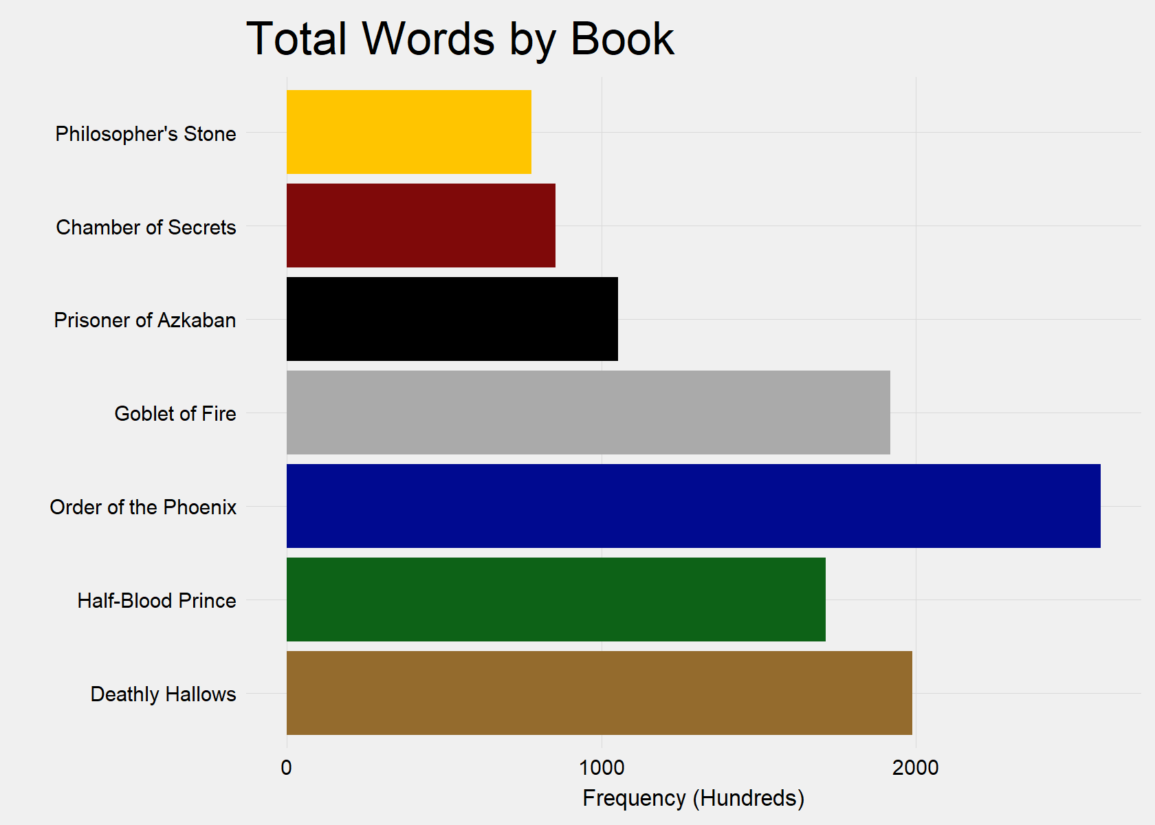

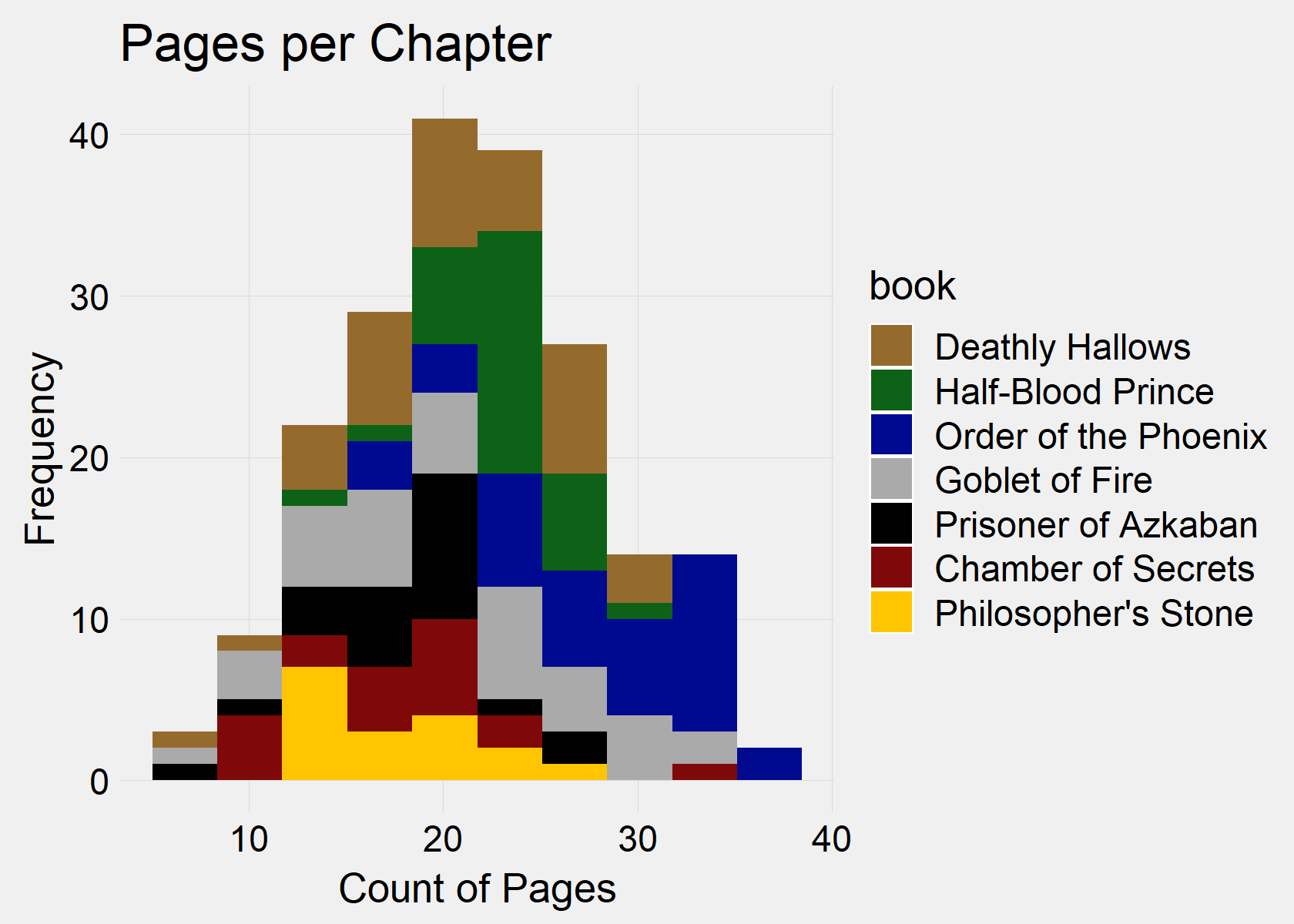
Word Distributions

Let’s look a little closer at the length of chapters. The average chapter in Harry Potter is over 5,000 words or 20 pages. The shortest book, Philosopher’s Stone (Book 1) also has the fewest average pages per chapter, while the longest book, Order of the Phoenix (Book 5) has the largest average pages per chapter.

# Word Count
df$totalwords <- sapply(strsplit(stripWhitespace(corpus), " "), length)

pasteNQ0("Average Amount of Words per Chapter")
summary(df$totalwords)

# Page Count
df$pagecount <- df$totalwords/250

# Raw Words by Book
df$words <- (strsplit(stripWhitespace(corpus), " "))

# Graph distribution of words all
ggplot(df, aes(totalwords, fill = I("maroon"))) + geom_histogram() + stat_bin(bins = 100) + 
    Grph_theme() + ylab("Frequency") + xlab("Count of Words") + ggtitle("Words per Chapter")

# Graph with book fill
ggplot(df, aes(pagecount, fill = book)) + geom_histogram() + stat_bin(bins = 10) + 
    scale_fill_manual(values = c("#946B2D", "#0D6217", "#000A90", "#AAAAAA", "#000000", 
        "#7F0909", "#FFC500")) + Grph_theme() + ylab("Frequency") + xlab("Count of Pages") + 
    ggtitle("Pages per Chapter") + theme(legend.position = "right")

[1] Average Amount of Words per Chapter
   Min. 1st Qu.  Median    Mean 3rd Qu.    Max. 
   1552    4208    5371    5396    6420    9081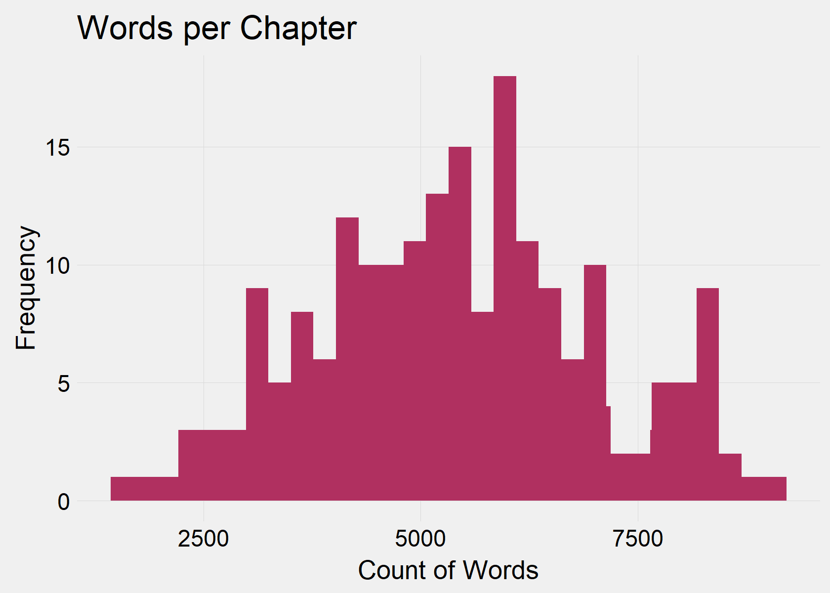 

Vocab Analysis

In order to better understand the maturity and reading level of each book, we will observe the breadth of vocabulary in each book. Below we look at counts of words and, more importantly, whether the vocab size grew or if words simply became more repetitive as the word count grew.

# Clean corpus
df$clean <- cleancorpus(df$text)

# Repair common stemmed words and character's names
df$clean <- str_replace_all(df$clean, "harri", "harry")
df$clean <- str_replace_all(df$clean, "hermion", "hermione")
df$clean <- str_replace_all(df$clean, "dumbledor", "dumbledore")
df$clean <- str_replace_all(df$clean, "tri", "try")
df$clean <- str_replace_all(df$clean, "voic", "voice")
df$clean <- str_replace_all(df$clean, "eye", "eyes")

[1] Set to lowercase
[1] Fixed contractions
[1] Removed punctuation, numbers, and other none characters
[1] Stripped whitespace
[1] Stemmed words

Definitions

• Total words are the amount of words regardless of repeated words
• Word count takes the number of unique “stemmed” words
• Vocab size is defined as the ratio of unique stemmed words relative to total words

Overall Vocab

# Raw text
corpustext <- df$clean %>% paste(collapse = "") %>% stripWhitespace()

# Total words
totalwords <- sapply(strsplit(stripWhitespace(corpustext), " "), length)
pasteNQ("Total Words:", totalwords)

# Unique words
uniquewords <- unlist(strsplit(stripWhitespace(corpustext), " ")) %>% unique() %>% 
    length()
pasteNQ("Unique Words:", uniquewords)

# Size of Vocab
vocabsize <- (uniquewords/totalwords)
vocabsize <- as.numeric(vocabsize) %>% round(2)
pasteNQ("Vocab Ratio:", vocabsize)

[1] Total Words: 1073007
[1] Unique Words: 35015
[1] Vocab Ratio: 0.03

Vocab by Book

Which book has a bigger vocab?

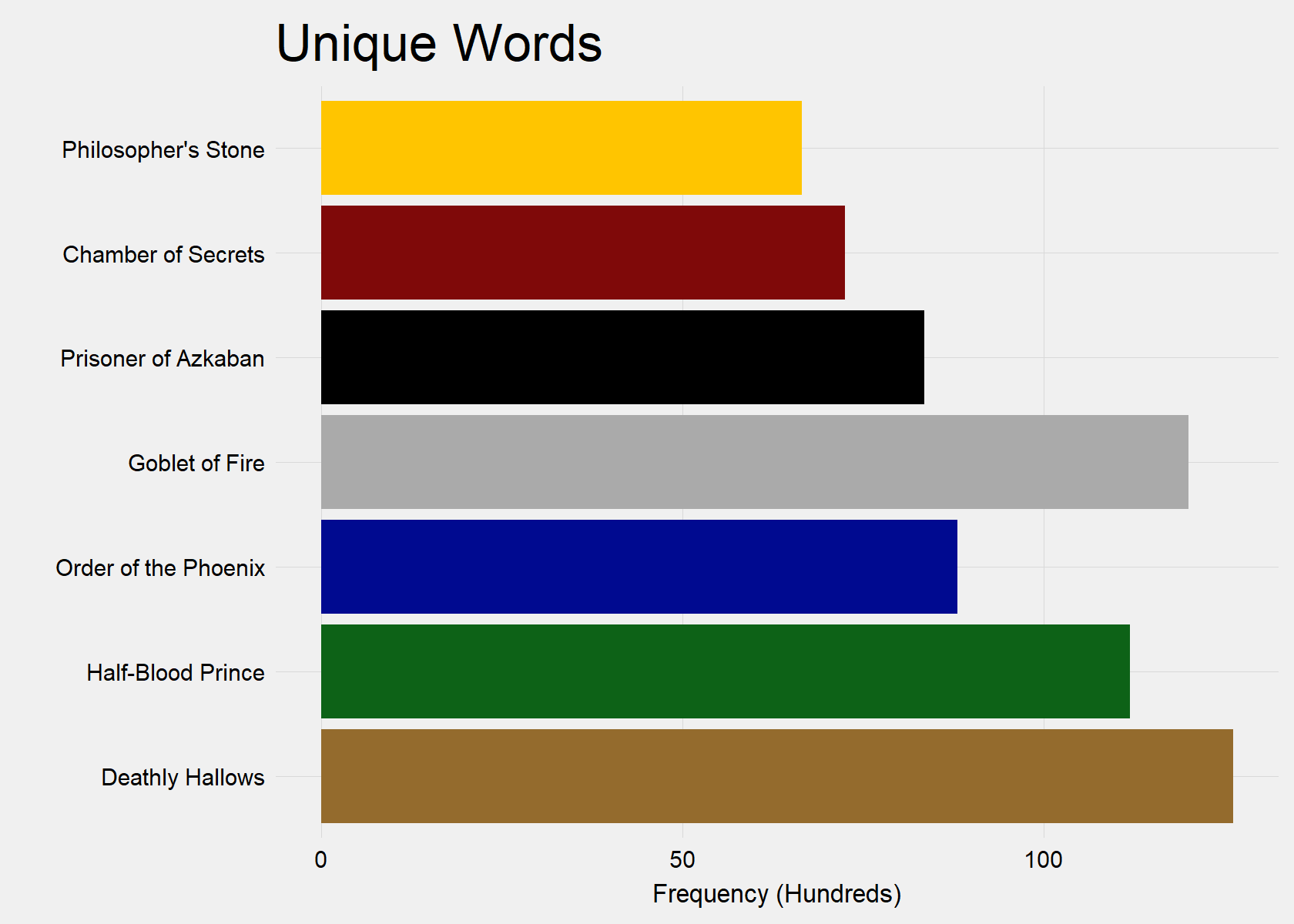
Below, we can see that the vocab increased in terms of unique words with each subsequent book. However, Goblet of Fire (Book 4) is a notable exception with the second most unique words. Deathly Hallows (Book 7) contains the most unique words.

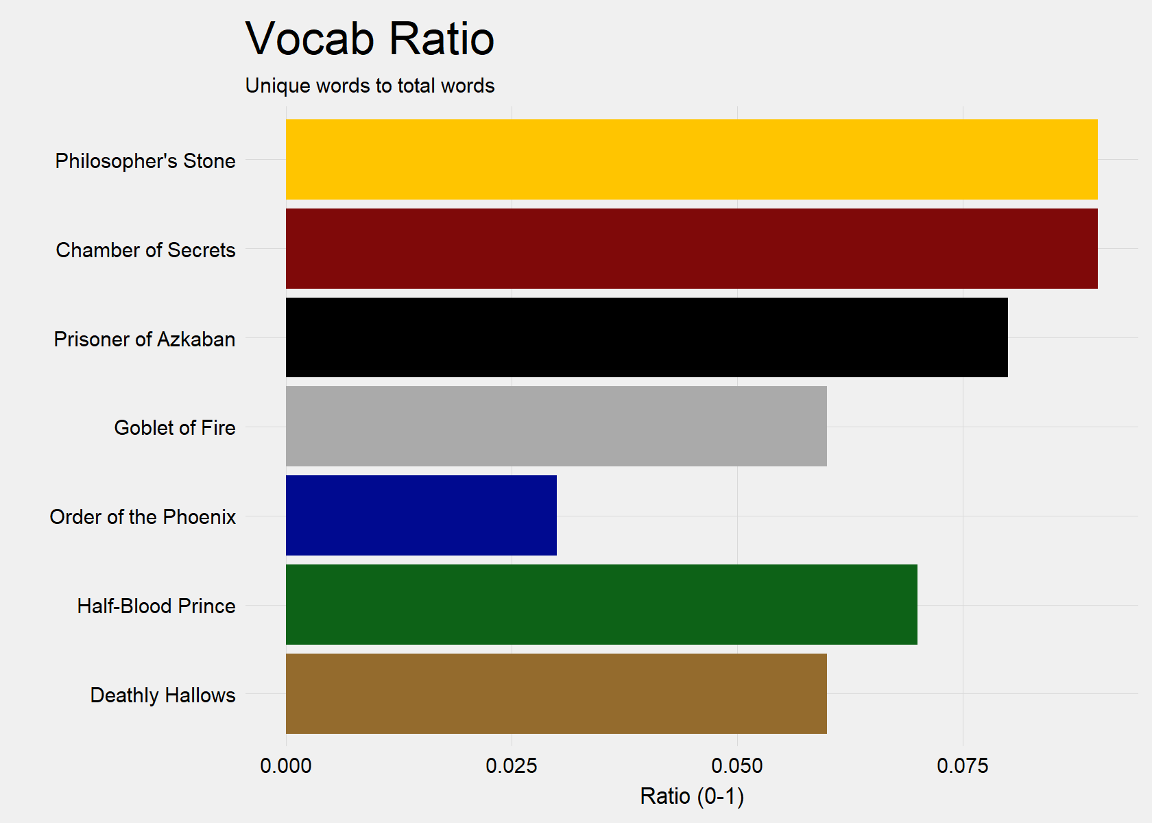
Further, we can see that the early books actually contained a more dense vocabulary as words were not repeated as frequently. This could be mainly due to their shorter total word count and less to do with their amount of unique works.

However, Order of the Phoenix (Book 5) appears to have the lowest density of vocabulary, because its unique word count is only fourth in the Series, despite easily containing the highest total word count. This indicates that Order of the Phoenix (Book 5) is the most repetitive in vocabulary.

# Words by Book
book_tf <- df[, c("clean", "book")] %>% unnest_tokens(word, clean, token = "words") %>% 
    group_by(book) %>% count(word) %>% arrange(desc(book))

# Total words Unique words Size of Vocab
i <- 1
book_words <- data.frame(book = NA, total = NA, unique = NA, vocab = NA)
for (t in titles) {
    assign(paste0("Book", i), book_tf[book_tf$book == t, "n"])
    assign("total", sum(get(paste0("Book", i))))
    assign("unique", nrow(get(paste0("Book", i))))
    assign("vocab", get("unique")/get("total"))
    assign("vocab", as.numeric(get("vocab")) %>% round(2))
    book_words <- rbind(book_words, c(t, get("total"), get("unique"), get("vocab")))
    i <- i + 1
}
book_words <- book_words[2:8, ]
book_words$book <- factor(book_words$book, levels = rev(titles))

# Graph
ggplot(book_words, aes(x = book, y = as.numeric(total)/1000, fill = book)) + geom_col() + 
    coord_flip() + Grph_theme_facet() + ylab("Frequency (Thousands)") + xlab("") + 
    ggtitle("Total Words") + scale_fill_manual(values = c("#946B2D", "#0D6217", "#000A90", 
    "#AAAAAA", "#000000", "#7F0909", "#FFC500")) + guides(fill = FALSE)

ggplot(book_words, aes(x = book, y = as.numeric(unique)/100, fill = book)) + geom_col() + 
    coord_flip() + Grph_theme_facet() + ylab("Frequency (Hundreds)") + xlab("") + 
    ggtitle("Unique Words") + scale_fill_manual(values = c("#946B2D", "#0D6217", 
    "#000A90", "#AAAAAA", "#000000", "#7F0909", "#FFC500")) + guides(fill = FALSE)

ggplot(book_words, aes(x = book, y = as.numeric(vocab), fill = book)) + geom_col() + 
    coord_flip() + Grph_theme_facet() + ylab("Ratio (0-1)") + xlab("") + ggtitle("Vocab Ratio") + 
    labs(subtitle = "Unique words to total words") + scale_fill_manual(values = c("#946B2D", 
    "#0D6217", "#000A90", "#AAAAAA", "#000000", "#7F0909", "#FFC500")) + guides(fill = FALSE)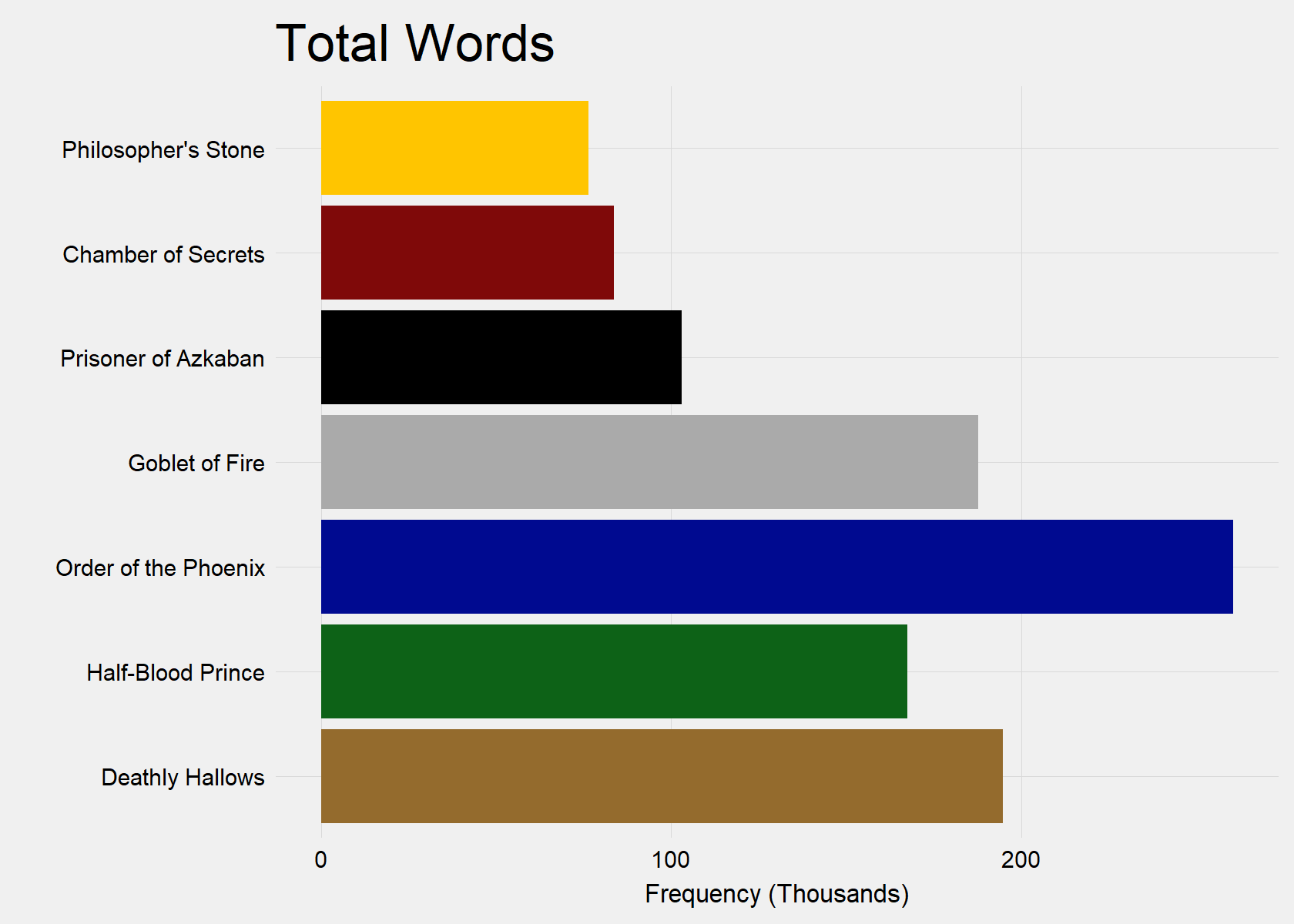

Subject matter

Term frequencies
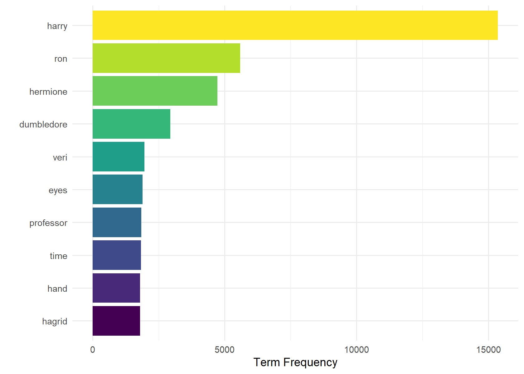
The easiest method for understand importance is examining term frequency (TF), which is the number of times a term (single word, in our case) appears. We removed stop words which are universally common words such as “the” and “said”. As characters are the most common terms after extensive stop word removal, it provides us an understanding of who are the most important characters.

The TF charts below shows that the most frequent word in every book is Harry. This is because there are perhaps one or two chapters in the whole series where Harry is not present. Therefore, other characters can be said to be mentioned in relation to Harry.

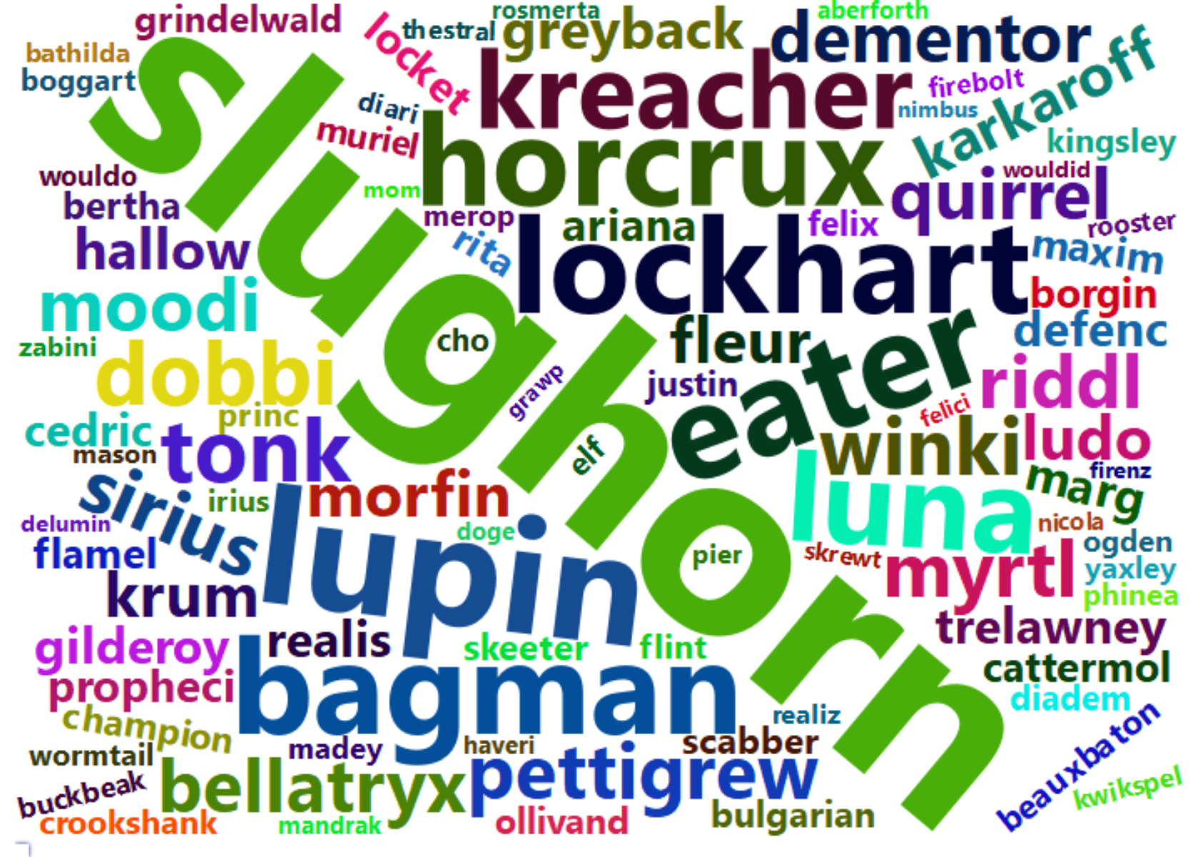
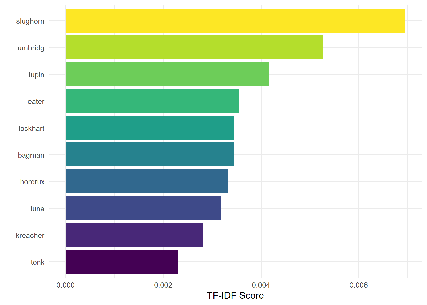
Term frequency-inverse document frequency scores
Term frequency-inverse document frequency (TF-IDF) analysis shows us which characters are mentioned the most within a book relative to across books. The technique involves scoring taking the TF multiplied by the IDF, which is calculated as the log of all documents (books) over the number of documents (books) containing the term. For example, “harry” would have a large TF but would contain an IDF of zero as it appears in every book.

The TF-IDF charts show that Professor Slughorn is the most specific character to a book. This means that he played a prominent role in Half-Blood Prince (Book 6), but was made few appearances in other books. Because Book 6 was his first appearance and only appeared a little in Book 7, his IDF score is very high. More interestingly, Reamus Lupin contains the third highest score, despite appearing early in the series in Prisoner of Azkaban (Book 3). This means that he is not prominent in many books, but when he is prominent (Book 3, Book 5, and Book 7), he is mentioned frequently.

Most Prominent Terms

# Remove Stopwords 
df$clean_sw <- removestopwords(df$clean, remove=c("said","c"))

# "Top Words using TF"
# TF Corpus
corpus_tf <- df %>%
  unnest_tokens("word", clean_sw, token="words") %>%
  anti_join(stop_words) %>% # remove larger amount of stop words
  count(word) %>%
  arrange(desc(n))

# Word Cloud of Most Common Words
wc <- wordcloud2(corpus_tf[1:300,], size = 1.3, gridSize = 14) 
embed_htmlwidget(wc)

# Bar Chart of Most Common Words
head(corpus_tf, 10) %>%
  mutate(word = factor(word, levels = rev(unique(word)))) %>%
  ggplot(aes(x=word, y=n, fill=word))+
    geom_col()+
    coord_flip()+
    theme_minimal()+
    scale_fill_viridis(discrete=T)+
    ylab("Term Frequency")+
    xlab("") + guides(fill=FALSE) 

# "Top Words using TF-IDF Scores"
# TF-IDF Corpus
corpus_tfidf <- df[,c("clean_sw","book")] %>%
  unnest_tokens(word, clean_sw, token="words") %>%
  anti_join(stop_words) %>% # remove larger amount of stop words
  group_by(book) %>%
  count(word) %>%
  bind_tf_idf(word, book, n) %>%
  group_by(word) %>%
  summarize(tf_idf=sum(tf_idf), n=sum(n), tf=sum(tf), idf=sum(idf)) %>%
  arrange(desc(tf_idf))

# Word Cloud of Most Common Words
wc <- wordcloud2(corpus_tfidf[1:100,], size = 0.9)
embed_htmlwidget(wc)

# Bar Chart of Most Common Words
head(corpus_tfidf, 10) %>%
  mutate(word = factor(word, levels = rev(unique(word)))) %>%
  ggplot(aes(x=word, y=tf_idf, fill=word))+
    geom_col()+
    coord_flip()+
    theme_minimal()+
    scale_fill_viridis(discrete=T)+
    ylab("TF-IDF Score")+
    xlab("") + guides(fill=FALSE) 

[1] Removed 177 stop words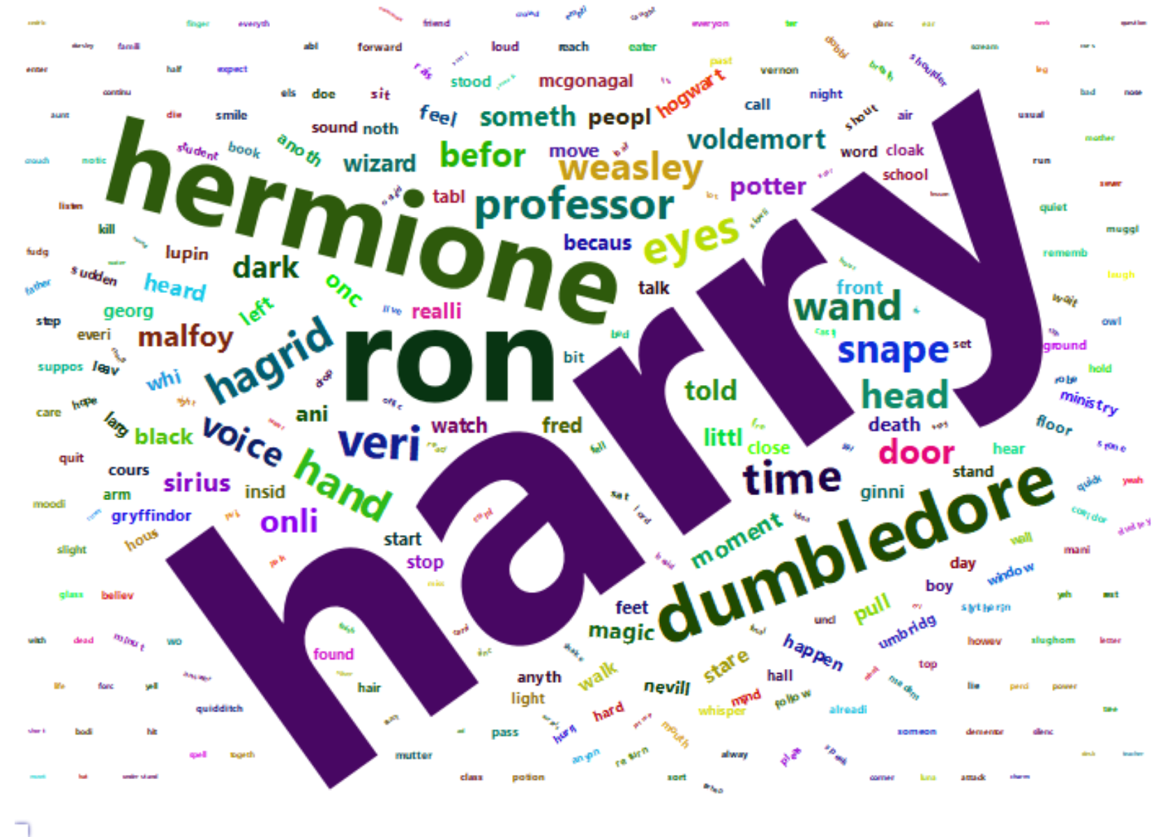

Terms by Book

This leads to a question that simple TFs by book can answer:

Who is Harry closest friend?

The Most Common Terms (TF) chart shows that, in nearly every book, Ron is mentioned more than Hermoine, indicating that he is Harry’s closest friend–although the movies may differ on this. However, it is worth noting that Hermoine does close this gap as the books progress and is mentioned more times in Deathly Hallows (Book 7). Interestingly, Professor Dumbledore jumps above Ron and Hermoined in Half-Blood Prince (Book 6), where he becomes more than a mentor and partners with Harry in the story’s main adventure.

I write “closest” instead of “best” as Ron is more prominent and, therefore, appears more “in Harry’s life.” However, some of these appearance can be (and are) of Ron fighting with Harry. Again, note that we can make this conclusion assuming that Ron and Hermoine appear in the books in relation to Harry. A book not written as from a single character’s perspective could not achieve these conclusions as easily.

Who are the most prominent secondary characters?

The TF chart can also help us understand who is the most prominent secondary character across books. Professor Dumbledore is the most frequently mentioned character after the three main characters (see the Most Used Terms charts in the previous section). The Most Common Terms (TF) chart below shows that he was not mentioned as much in the first three books, but became very prominent by Goblet of Fire (Book 4).

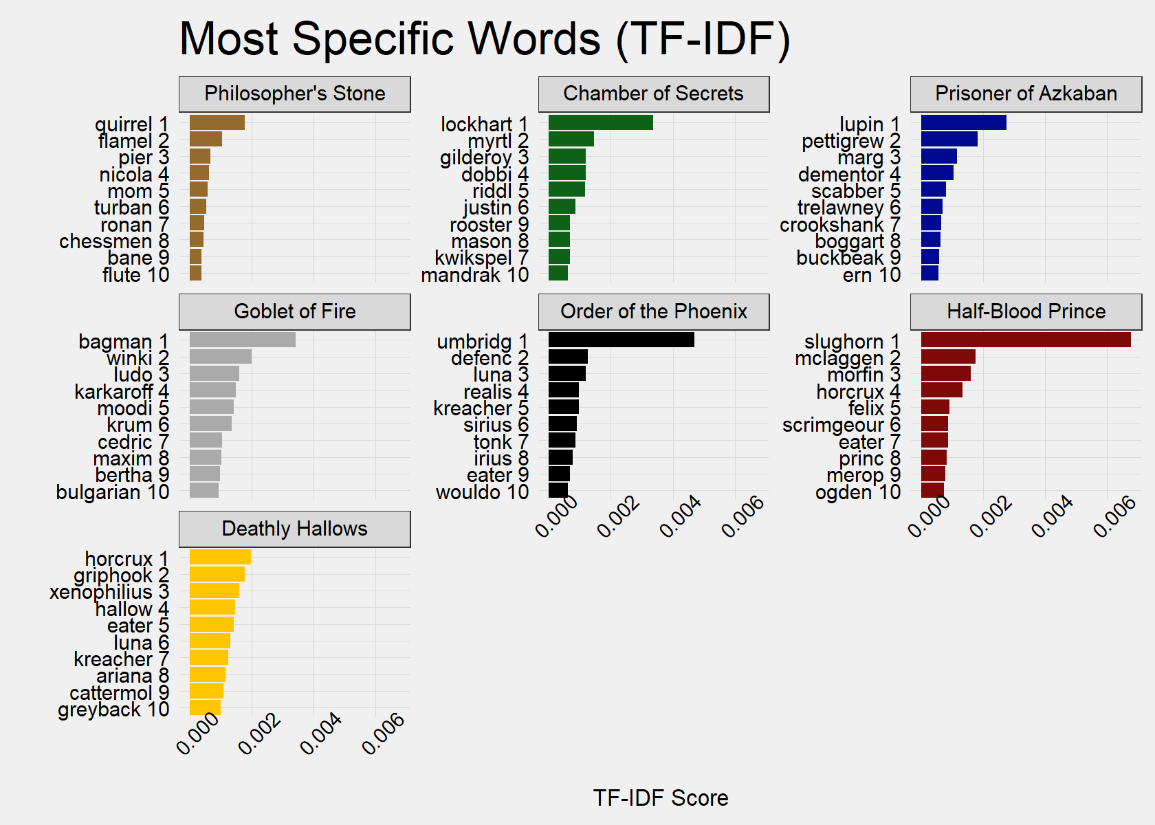
TF-IDF provides us with a proxy for secondary characters specific to a certain book: characters important in certain books, but not in every book. Therefore, we are not searching for secondary characters who are consistently present throughout the series, such as Hagrid or Dumbledore.

In the Most Specific Words (TF-IDF) chart, we can see an obvious pattern: the most prominent secondary character is the new teacher at Hogwarts in 5 of the 7 books. Four of these times, the new teacher is the Defense Against the Dark Arts teacher. Interestly, Professor Moody, the Defense Against Dark Arts teacher, is only ranked fifth in Goblet of Fire (Book 4). This is likely because there are many important characters specific to that book and that Mad-Eye Moody remains prominent after Book 4.

# TF
book_tf <- df[,c("clean_sw","book")] %>%
  unnest_tokens(word, clean_sw, token="words") %>%
  anti_join(stop_words) %>% # remove larger amount of stop words
  group_by(book) %>%
  count(word) %>%
  arrange(desc(n), .by_group=T)

# TF-IDF
book_tf_idf <- df[,c("clean_sw","book")] %>%
  unnest_tokens(word, clean_sw, token="words") %>%
  anti_join(stop_words) %>% # remove larger amount of stop words
  group_by(book) %>%
  count(word) %>%
  bind_tf_idf(word, book, n) %>%
  arrange(desc(tf_idf), .by_group=F)

# Bar Chart of Most Common Words
top_n(book_tf, 10, n) %>% 
  mutate(order = row_number()) %>%
  ungroup %>%
  arrange(book, n) %>%
  mutate(label = paste(book, order, word),
         book = factor(book, levels = titles)) %>%  
  mutate(labels = factor(label, levels = label,
                         label = paste(word, order))) %>%
    ggplot(aes(x=reorder(labels,rev(order)), y=n, fill=book))+
    facet_wrap(~ book, scales = "free_y") +
    geom_col()+
    coord_flip()+
    scale_fill_manual(values = c("#946B2D", "#0D6217", "#000A90", 
                                 "#AAAAAA", "#000000", "#7F0909", "#FFC500")) +
    Grph_theme_facet()+
    theme(axis.text.x=element_text(size=8, angle=45)) +
    ylab("Term Frequency")+
    xlab("") + ggtitle("Most Common Words (TF)") +
    guides(fill=FALSE) 

# Bar Chart of Most Specific Words
top_n(book_tf_idf, 10, tf_idf) %>% 
  mutate(order = row_number()) %>%
  ungroup %>%
  arrange(book, tf_idf) %>%
  mutate(label = paste(book, order, word),
         book = factor(book, levels = titles)) %>%  
  mutate(labels = factor(label, levels = label,
                         label = paste(word, order))) %>%
    ggplot(aes(x=labels, y=tf_idf, fill=book))+
    ylab(word) +
    facet_wrap(~ book, scales = "free_y") +
    geom_col()+
    coord_flip()+
    scale_fill_manual(values = c("#946B2D", "#0D6217", "#000A90", 
                                 "#AAAAAA", "#000000", "#7F0909", "#FFC500")) +
    Grph_theme_facet()+
    theme(axis.text.x=element_text(angle=45)) +
    ylab("TF-IDF Score")+
    xlab("") + ggtitle("Most Specific Words (TF-IDF)") + 
    guides(fill=FALSE)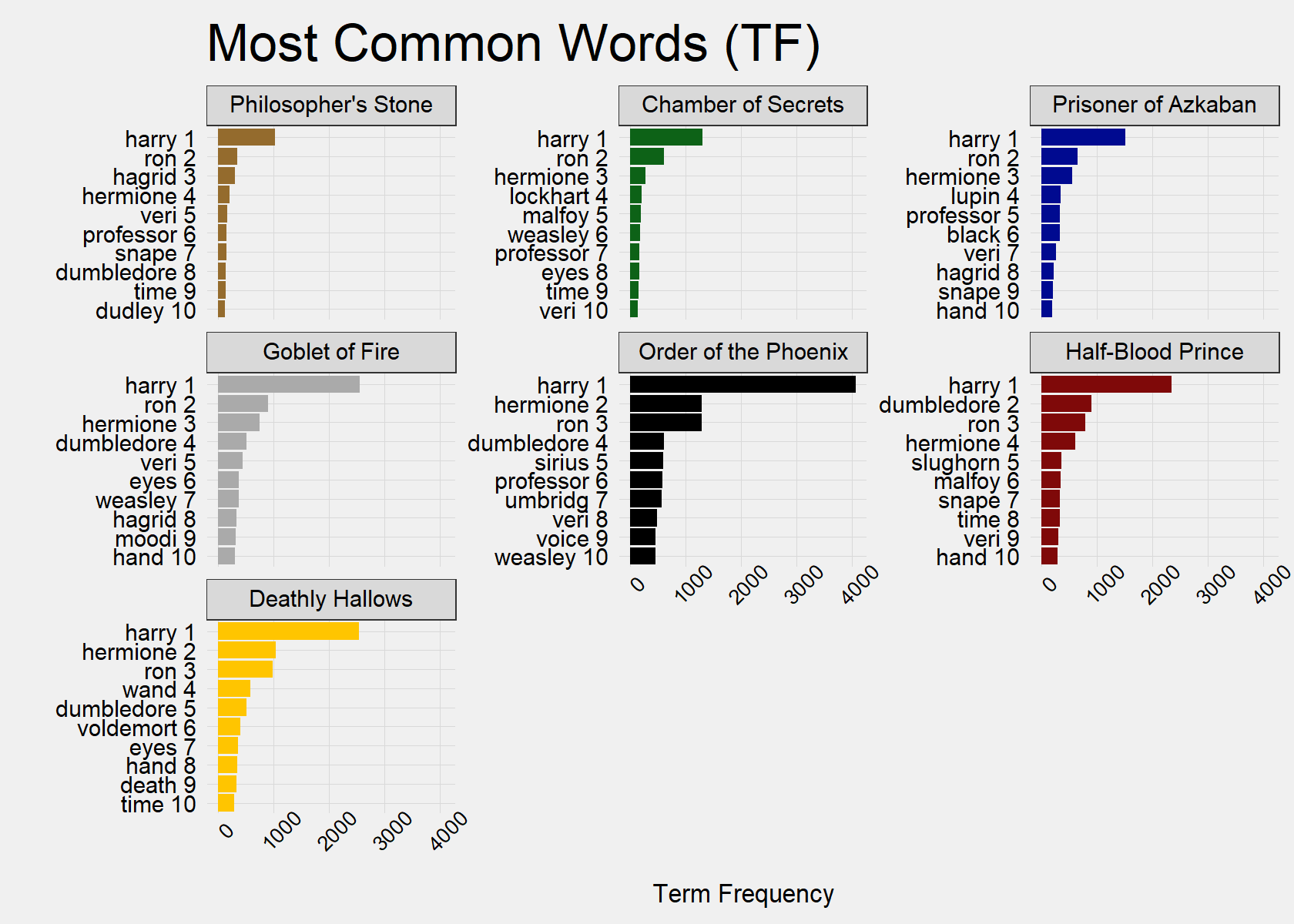 

Topic Analysis

Finally, let’s use structural topic modeling to answer:

What are the 4 major themes/settings in the Series?

By using chapters as the level analysis, we are only observing these themes/settings at an extremely broad level

With topic analysis, at only 4 topics, the major themes/settings appear to be:

• Topic 1) The Muggle world
  • These chapters tend to be early in the early of book such as Harry’s summers with the Dursleys
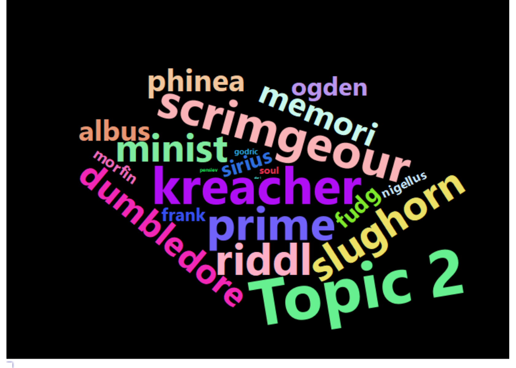
• Topic 2) The magical community outside of Hogwarts
  • Involves Ministry of Magic, journalists, and others in the Wizarding world outside of Hogwarts
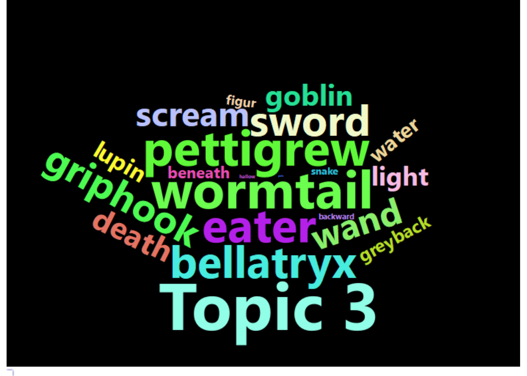
• Topic 3) Voldemort’s story arch
  • These chapters tend to be in later books, involving pursuit of horcruxes, run-ins with villians, and magical objects
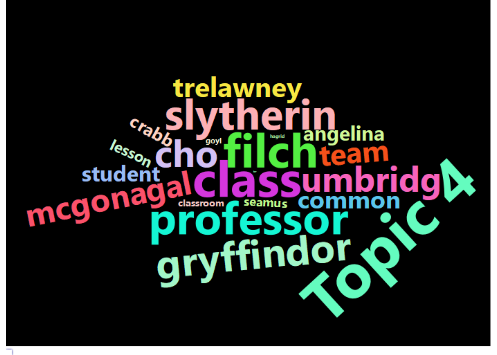
• Topic 4) Hogwarts classroom/Quidditch field
  • These chapters tend to be in the middle of the books in which Harry and his friends are at Hogwarts, spending time studying and playing Quidditch

Document Term Matrix

set.seed(0)

# tokenize
it <- itoken(df$clean_sw, ids = df$id, progressbar = FALSE)

# ngrams
vocab <- create_vocabulary(it, ngram)
vocab <- prune_vocabulary(vocab, term_count_min = 5L)

vectorizer <- vocab_vectorizer(vocab)

# create dtm
dtm <- create_dtm(it, vectorizer, type = "dgCMatrix")

# number of term input
pasteNQ("document term matrix specifications:")
pasteNQ("cleaned", totalwords, "words into", ncol(dtm))
pasteNQ("number of documents:", nrow(dtm))

[1] document term matrix specifications:
[1] cleaned 1073007 words into 6417
[1] number of documents: 200

Word Cloud by Topic

# Convert DTM to list
documents <- apply(as.matrix(dtm), 1, function(y) {
      rbind(which(y > 0), as.integer(y[y > 0])) 
})
processed <- list(documents=documents, vocab=vocab$term)

# Prep documents for stm package
out <- prepDocuments(processed$documents, processed$vocab, lower.thresh = 3, verbose=F)

stmmodel <- stm(documents = out$documents, vocab = out$vocab,
                K = K,
                max.em.its = 500, 
                # data = out$meta,
                init.type = "Spectral", 
                verbose=F)

# List defining words for each topic
topics <- labelTopics(stmmodel, 1:K, n=20)
for (i in 1:K) {
  frex <- data.frame(words=topics$frex[i,], n=21-seq(topics$frex[i,]), stringsAsFactors=F)
  frex$words <- str_replace_all(frex$words, "_", " ")
  clouds <- data.frame(words = c(frex$words, 
                                 paste("Topic",i)), 
                       weight = c(frex$n, 25))
  assign(paste0("wc_", i), (wordcloud2(clouds, size=0.5,
        color = "random-light", backgroundColor = "black")))
}
embed_htmlwidget(wc_1)
embed_htmlwidget(wc_2)
embed_htmlwidget(wc_3)
embed_htmlwidget(wc_4)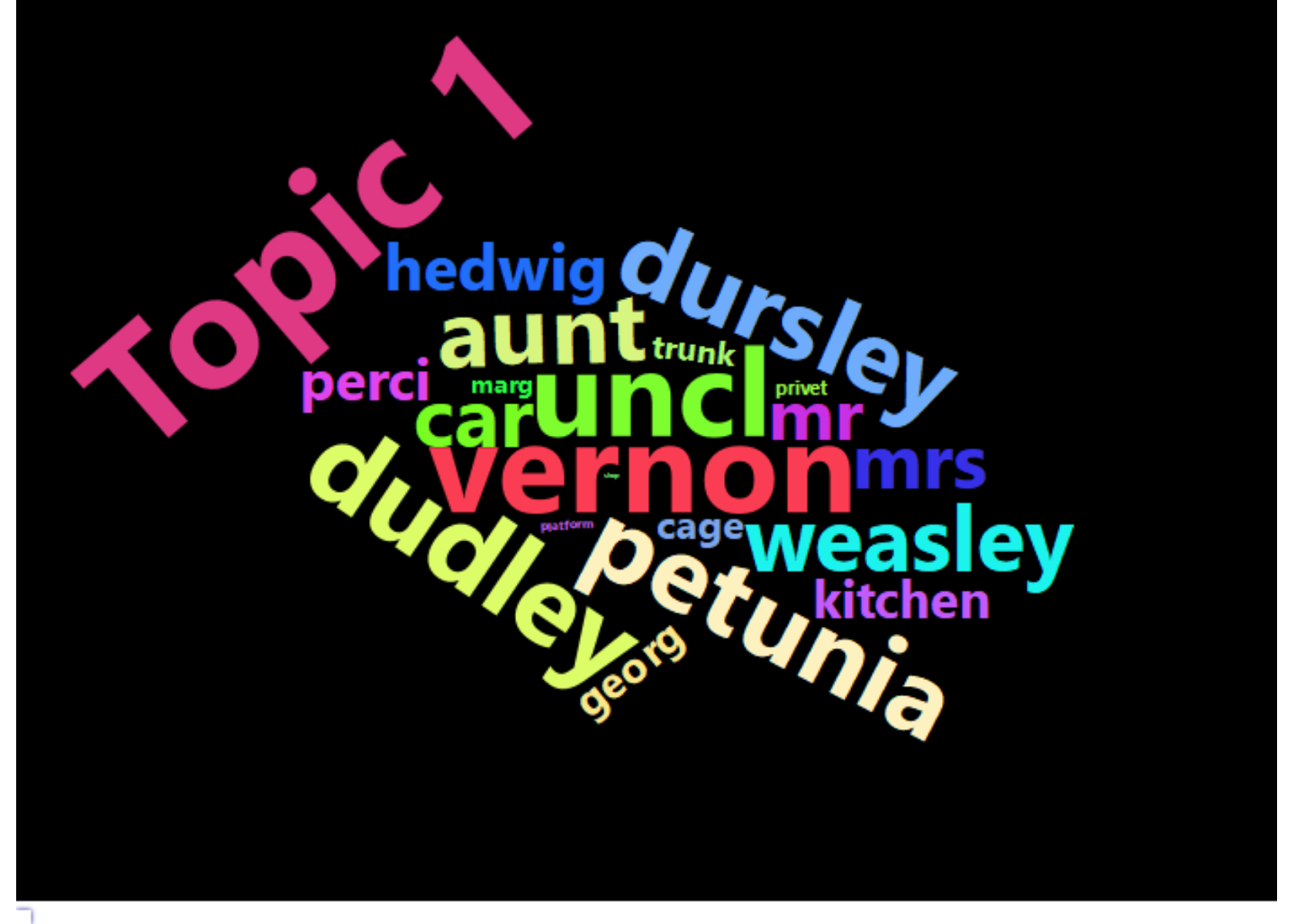

Chapters Represented in Topic

Below are the first sentences of each chapter most associated with each topic and therefore most representive of each topic.

for (i in 1:K) {
    assign("quotes", findThoughts(stmmodel, texts = pasteNQ0(df$book, " (Chapter ", 
        df$chapter, "): ", sentences$beginning), n = 3, topics = i)$docs[[1]])
    print(pasteNQ("Topic", i, "Example"))
    print(get("quotes")[1])
    print(get("quotes")[2])
    print(get("quotes")[3])
    cat("\n")
}

[1] Topic 1 Example
[1] Philosopher's Stone (Chapter 3): THE LETTERS FROM NO ONE  The escape of the Brazilian boa constrictor earned Harry his longest-ever punishment. By the time he was allowed out of his cupboard again, the summer holidays had started and Dudley had already broken his new video camera, c ...  
[1] Prisoner of Azkaban (Chapter 2):   AUNT MARGE'S BIG MISTAKE  Harry went down to breakfast the next morning to find the three Dursleys already sitting around the kitchen table. They were watching a brand-new television, a welcome-home-for-the-summer present for Dudley, who had been c ...    
[1] Chamber of Secrets (Chapter 3): THE BURROW  Ron.l" breathed Harry, creeping to the window and pushing it up so they could talk through the bars. "Ron, how did you - What the -?"  Harry's mouth fell open as the full impact of what he was seeing hit him. Ron was leaning out of the ba ...    

[1] Topic 2 Example
[1] Half-Blood Prince (Chapter 23):  Harry could feel the Felix Felicis wearing off as he creeped back into the castle. The front door had remained un locked for him, but on the third floor he met Peeves and only narrowly avoided detection by diving sideways through one of his shortcut ...
[1] Half-Blood Prince (Chapter 1):  It was nearing midnight and the Prime Minister was sitting alone in his office, reading a long memo that was slipping through his brain without leaving the slightest trace of meaning behind. He was waiting for a call from the President of a far dist ...
[1] Deathly Hallows (Chapter 18): The sun was coming up: The pure, colorless vastness of the sky stretched over him, indifferent to him and his suffering. Harry sat down in the tent entrance and took a deep breath of clean air. Simply to be alive to watch the sun rise over the sparkl ...

[1] Topic 3 Example
[1] Order of the Phoenix (Chapter 35): Beyond the VeilBlack shapes were emerging out of thin air all around them, blocking their way left and right; eyes glinted through slits in hoods, a dozen lit wand tips were pointing directly at their hearts; Ginny gave a gasp of horror.    'To me, P ...
[1] Goblet of Fire (Chapter 34):    Wormtail approached Harry, who scrambled to find his feet, to support his own weight before the ropes were untied. Wormtail raised his new silver hand, pulled out the wad of material gagging Harry, and then, with one swipe, cut through the bonds t ...  
[1] Goblet of Fire (Chapter 32):    Harry felt his feet slam into the ground; his injured leg gave way, and he fell forward; his hand let go of the Triwizard Cup at last. He raised his head.  "Where are we?" he said.  Cedric shook his head. He got up, pulled Harry to his feet, and t ...      

[1] Topic 4 Example
[1] Prisoner of Azkaban (Chapter 15):   THE QUIDDITCH FINAL  He sent me this," Hermione said, holding out the letter.  Harry took it. The parchment was damp, and enormous teardrops had smudged the ink so badly in places that it was very difficult to read.  Dear Hermione, We lost. I'm all ...        
[1] Philosopher's Stone (Chapter 11): QUIDDITCH  As they entered November, the weather turned very cold. The mountains around the school became icy gray and the lake like chilled steel. Every morning the ground was covered in frost. Hagrid could be seen from the upstairs windows defrosti ...  
[1] Order of the Phoenix (Chapter 19): The Lion and the SerpantHarry felt as though he were carrying some kind of talisman inside his chest over the following two weeks, a glowing secret that supported him through Umbridge's classes and even made it possible for him to smile blandly as he ...

Next Steps

This was an extremely broad and high level look at Harry Potter. Subsequent analysis look more in depth at the tone of the heros and villians and comparisons of the books to the films (upcoming).